Fashion MNIST with LightGBM and ConvNet
Follow along on Google Colab.
Introduction
Image classification is the task of categorizing images into different classes. There are many use cases for image classification. For example:
In practice, the biggest challenge in image classification is the collection of labeled data. However, in this exercise, the popular Fashion MNIST dataset was used to showcase different techniques that can be used for image classification.
This exercise was originally done as part of a course assignment for Big Data Analytics (IST 718) at Syracuse University.
Fashion MNIST Dataset
The Fashion MNIST dataset is an alternative to the popular digit MNIST dataset. This dataset contains 70,000 28x28 grayscale images in 10 fashion categories. 60,000 of which are in the train set, and 10,000 of which are in the test set. The dataset can be obtained here. It can also be retrieved through the TensorFlow’s API.
The 10 fashion categories in the Fashion MNIST dataset:
| Label | Description |
|---|---|
| 0 | T-shirt/top |
| 1 | Trouser |
| 2 | Pullover |
| 3 | Dress |
| 4 | Coat |
| 5 | Sandal |
| 6 | Shirt |
| 7 | Sneaker |
| 8 | Bag |
| 9 | Ankel boot |
The Fashion MNIST dataset is a perfectly balanced dataset with even number of observations per class.
Set Up
This notebook uses cuDF and cuML by RAPIDS, and it’s designed to run on Google Colab.
Install RAPIDS 0.18
This clones the Github Repository for RAPIDS and uses a bash script to install RAPIDS on Google Colab.
!git clone https://github.com/rapidsai/rapidsai-csp-utils.git
!bash rapidsai-csp-utils/colab/rapids-colab.sh 0.18
import sys, os

dist_package_index = sys.path.index('/usr/local/lib/python3.7/dist-packages')
sys.path = sys.path[:dist_package_index] + ['/usr/local/lib/python3.7/site-packages'] + sys.path[dist_package_index:]
sys.path
exec(open('rapidsai-csp-utils/colab/update_modules.py').read(), globals())
Install LightGBM
This install the GPU version of LightGBM on Google Colab. LightGBM is a Gradient Boosting Tree-based Model developed by Microsoft.
%pip install lightgbm --install-option=--gpu
Import Packages
# tensorflow
from tensorflow.keras.datasets import fashion_mnist
from tensorflow import keras
from tensorflow.keras import layers

# data manipulation
import cudf
import numpy as np # could also try using cupy

# additional models
from cuml.manifold import TSNE # t-distributed stochastic neighbor embedding
import cuml
import lightgbm as lgb
from sklearn.preprocessing import label_binarize
from sklearn.metrics import (roc_curve, auc, roc_auc_score, confusion_matrix,
                             precision_score, recall_score, accuracy_score)

# visuals
import matplotlib as mpl
import matplotlib.pyplot as plt
import seaborn as sns
from ipywidgets import interact
import ipywidgets as widgets
Data
The 10 labels in the Fashion MNIST dataset ordered by their index number.
label_index = [
    'T-shirt/top',
    'Trouser',
    'Pullover',
    'Dress',
    'Coat',
    'Sandal',
    'Shirt',
    'Sneaker',
    'Bag',
    'Ankel boot'
]
Load Data from TensorFlow
(X_train, y_train), (X_test, y_test) = fashion_mnist.load_data()

X_train = X_train.astype("float32") / 255
X_test = X_test.astype("float32") / 255

y_test_binarize = label_binarize(y_test, classes=list(range(10)))
Exploratory Data Analysis
Visualize the Dataset
This script below was taken from Kaggle and it was used to visualize the digit MNIST dataset. It works just fine for the Fashion MNIST dataset.
def plot_MNIST(instances, images_per_row=10):
    size = 28
    images_per_row = min(len(instances), images_per_row)
    images = [instance.reshape(size,size) for instance in instances]
    n_rows = (len(instances) - 1) // images_per_row + 1
    row_images = []
    n_empty = n_rows * images_per_row - len(instances)
    images.append(np.zeros((size, size * n_empty)))
    for row in range(n_rows):
        rimages = images[row * images_per_row : (row + 1) * images_per_row]
        row_images.append(np.concatenate(rimages, axis=1))
    image = np.concatenate(row_images, axis=0)
    plt.imshow(image, cmap = mpl.cm.binary)
    plt.axis("off")
plt.figure(figsize=(9,9))
example_images = X_train[:25]
plot_MNIST(example_images, images_per_row=5)
plt.show()
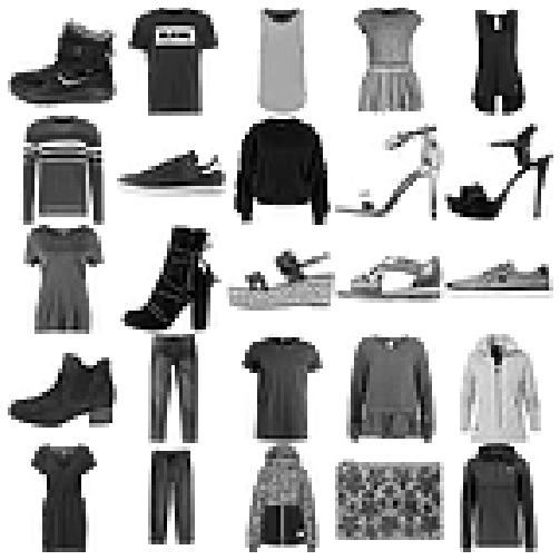
Figure above shows 25 sample images from the fashion MNIST dataset. There are a variety of different appeals in the dataset for each category.
T-Distributed Stochastic Neighbor Embedding (tSNE)
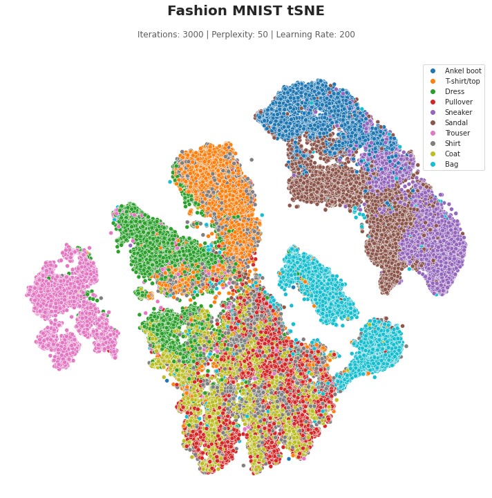
tSNE is a popular visualization tool to visualize high dimensional dataset. It is perfect for Fashion MNIST as it has 784 features. This is done using the cuML library.
def tsne_plot(b):

  # output.clear_output()

  _n_iter = n_iter.value
  _perplexity = perplexity.value
  _learning_rate = learning_rate.value

  tsne = TSNE(
      n_components=2,
      n_neighbors=4*_perplexity,
      perplexity=_perplexity,
      learning_rate=_learning_rate,
      n_iter=_n_iter,
      random_state=718)

  data_tsne = tsne.fit_transform(X_train.reshape(X_train.shape[0], -1))

  f, ax = plt.subplots(figsize=(10, 10))

  with sns.axes_style("white"):
      sns.despine(f, left=True, bottom=True)

      g = sns.scatterplot(
          x = data_tsne[:,0],
          y = data_tsne[:,1],
          hue = [label_index[int(val)] for val in y_train],
          ax = ax
      )

      ax.text(x=0.5, y=1.1, s='Fashion MNIST tSNE', fontsize=20, weight='bold', ha='center', va='bottom', transform=ax.transAxes)
      ax.text(x=0.5, y=1.05, s=f'Iterations: {_n_iter} | Perplexity: {_perplexity} | Learning Rate: {_learning_rate}', fontsize=12, alpha=0.75, ha='center', va='bottom', transform=ax.transAxes)

      g.set(xticklabels=[])
      g.set(yticklabels=[])
      g.tick_params(left=False, bottom=False)

      f.tight_layout()
  with output:
      output.clear_output()
      g
ipywidgets was used to showcase how one could use it as a tool to determine how different parameters affect the tSNE model.
style = {'description_width': 'initial'}
layout = {'width':'500px'}

n_iter = widgets.IntSlider(
    value=3000, min=500, max=3000, step=100,
    description='Number of Iterations:', style=style, layout=layout)
perplexity = widgets.IntSlider(
    value=50, min=10, max=100, step=10,
    description='Perplexity:', style=style, layout=layout)
learning_rate = widgets.IntSlider(
    value=200, min=100, max=300, step=20,
    description='Learning Rate:', style=style, layout=layout)

run_tsne = widgets.Button(description='Run tSNE')
output = widgets.Output()
run_tsne.on_click(tsne_plot)

control = widgets.VBox([n_iter,
                        perplexity,
                        learning_rate,
                        run_tsne])
display(control, output)

From the tSNE figure above, it appears that trousers and bags can be easily differentiated from the other apparels. The three footwears, ankle boots, sneakers and sandals are separated from the rest of the apparels into its own cluster while maintaining some separation between each other. Pullover, shirt and coat are all clustered together which suggest that it could be difficult to classify them. Shirt, in particular, look somewhat dispersed.
Models
Two classification models were created to classify the Fashion MNIST images. They are LightGBM by Microsoft and ConvNet by Keras (TensorFlow).
Both models were trained with a conventional train-test split.
LightGBM
Using a DART booster and a multiclass logistic loss function, LightGBM was able to achieve an 88.9% testing accuracy. This accuracy was achieved with the default parameters with no changes to the number of bins, leaves, iterations or learning rate. As LightGBM supports computation on GPU, this model was trained with an NVIDIA Tesla T4. The computational performance was acceptable, completing in just 1 minutes and 40 seconds.
Additional information on LightGBM is below:
Training
%%time
lgb_params = dict(
    boosting='dart',
    objective='multiclass',
    metrics='multi_logloss',
    verbose=1,
    random_state=718,
    device='gpu',
    num_class=len(label_index)
)


lgb_train = lgb.Dataset(X_train.reshape(X_train.shape[0], -1), y_train)
lgb_test = lgb.Dataset(X_test.reshape(X_test.shape[0],-1), y_test, reference=lgb_train)

lgb_model = lgb.train(lgb_params, lgb_train)
Prediction
# Train
y_prob_lgb_train = lgb_model.predict(X_train.reshape(X_train.shape[0], -1))
y_pred_lgb_train = [np.argmax(row) for row in y_prob_lgb_train]

# Test
y_prob_lgb = lgb_model.predict(X_test.reshape(X_test.shape[0],-1))
y_pred_lgb = [np.argmax(row) for row in y_prob_lgb]
Performance
Training versus Testing
print(f"""LightGBM Performance on Train Set
Accuracy: {round(accuracy_score(y_train, y_pred_lgb_train),3)}
Precision (weighted): {round(precision_score(y_train, y_pred_lgb_train, average='weighted'),3)}
Recall (weighted): {round(recall_score(y_train, y_pred_lgb_train, average='weighted'),3)}""")
print(f"""LightGBM Performance on Test Set
Accuracy: {round(accuracy_score(y_test, y_pred_lgb),3)}
Precision (weighted): {round(precision_score(y_test, y_pred_lgb, average='weighted'),3)}
Recall (weighted): {round(recall_score(y_test, y_pred_lgb, average='weighted'),3)}""")
| LightGBM Performance | Train | Test |
|---|---|---|
| Accuracy | 95.8% | 88.9% |
| Precision (Weighted) | 95.8% | 88.9% |
| Recall (Weighted) | 95.8% | 88.9% |
Confusion Matrix
f, ax = plt.subplots(figsize=(10, 7))

conf_mat = confusion_matrix(y_test, y_pred_lgb)
sns.heatmap(conf_mat, xticklabels=label_index, yticklabels=label_index,
            annot=True, annot_kws={"size": 16}, fmt='d', cbar=False, ax=ax)

ax.text(x=0.5, y=1.05, s='LightGBM - Confusion Matrix', fontsize=20, weight='bold', ha='center', va='bottom', transform=ax.transAxes)
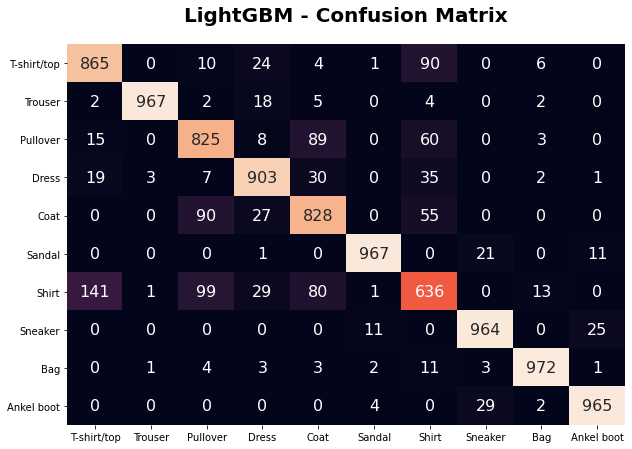
The confusion matrix shows that the model was capable to predict most of the fashion categories. It struggles with “shirt”, as it was suggested by the tSNE analysis. Shirt and T-shirt, in particular, has the highest misclassification rate between each other.
ROC
fpr = dict()
tpr = dict()
roc_auc = dict()

for i, label in enumerate(label_index):
    fpr[i], tpr[i], _ = roc_curve(y_test_binarize[:, i], y_prob_lgb[:, i])
    roc_auc[i] = auc(fpr[i], tpr[i])

fpr["micro"], tpr["micro"], _ = roc_curve(y_test_binarize.ravel(), y_prob_lgb.ravel())
roc_auc["micro"] = auc(fpr["micro"], tpr["micro"])

all_fpr = np.unique(np.concatenate([fpr[i] for i in range(10)]))
mean_tpr = np.zeros_like(all_fpr)

for i in range(10):
    mean_tpr += np.interp(all_fpr, fpr[i], tpr[i])

mean_tpr /= 10

fpr["macro"] = all_fpr
tpr["macro"] = mean_tpr
roc_auc["macro"] = auc(fpr["macro"], tpr["macro"])

# Plot all ROC curves
plt.figure(figsize=(8,8))
plt.plot(fpr["micro"], tpr["micro"],
         label='micro-average ROC curve (area = {0:0.2f})'
               ''.format(roc_auc["micro"]),
         color='deeppink', linestyle=':', linewidth=4)

plt.plot(fpr["macro"], tpr["macro"],
         label='macro-average ROC curve (area = {0:0.2f})'
               ''.format(roc_auc["macro"]),
         color='navy', linestyle=':', linewidth=4)

for i, label in enumerate(label_index):
    plt.plot(fpr[i], tpr[i], lw=2,
             label=f'{label} (area = {round(roc_auc[i],2)})')

plt.plot([0, 1], [0, 1], 'k--', lw=2)
plt.xlim([0.0, 1.0])
plt.ylim([0.0, 1.05])
plt.xlabel('False Positive Rate')
plt.ylabel('True Positive Rate')
plt.title('LightGBM - ROC curves of individual classes in Fashion MNIST')
plt.legend(loc="lower right")
plt.show()
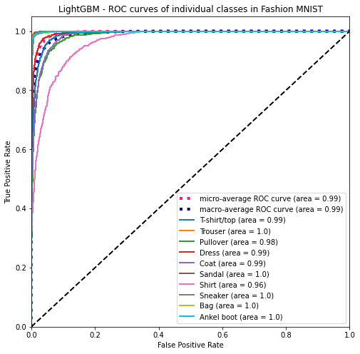
The LightGBM model’s ROC curve for each of the ten categories in the Fashion MNIST dataset. With a 0.96 AUC, shirt is the worse of the ten categories.
Keras ConvNet
A 7 layers sequential ConvNet was created:
- Convolutional Layer with 32 filters and a (3,3) filter size. This layer uses the rectified linear activation function.
- Max pooling layer
- Convolutional Layer with 64 filters and a (3,3) filter size. This layer uses the rectified linear activation function.
- Max pooling layer
- Flatten
- Dropout with 50% probability
- Dense layer with 10 nodes. This layer uses the softmax activation function.
The ConvNet uses a stochastic gradient descent optimizer with a 0.01 learning rate and a momentum of 0.9 and trained with a multiclass logistic loss function (categorical cross-entropy). 10% of the training data was held back for validation to avoid data leakage. With a batch size of 128, and an epoch of 15, the model was trained in 53.8s.
Keras’s ConvNet was able to achieve an 88.8% testing accuracy.
Training
X_train_keras = np.expand_dims(X_train, -1)
X_test_keras = np.expand_dims(X_test, -1)

y_train_keras = keras.utils.to_categorical(y_train, 10)
y_test_keras = keras.utils.to_categorical(y_test, 10)
keras_model = keras.Sequential(
    [
        keras.Input(shape=(28, 28, 1)),
        layers.Conv2D(32, kernel_size=(3, 3), activation="relu"),
        layers.MaxPooling2D(pool_size=(2, 2)),
        layers.Conv2D(64, kernel_size=(3, 3), activation="relu"),
        layers.MaxPooling2D(pool_size=(2, 2)),
        layers.Flatten(),
        layers.Dropout(0.5),
        layers.Dense(10, activation="softmax"),
    ]
)

keras_model.summary()
%%time
keras_model.compile(loss="categorical_crossentropy",
                    optimizer=keras.optimizers.SGD(lr=0.01, momentum=0.9),
                    metrics=["accuracy"])
keras_model.fit(X_train_keras, y_train_keras, batch_size=128, epochs=15, validation_split=0.1)
Prediction
# Train
y_prob_keras_train = keras_model.predict(X_train_keras)
y_pred_keras_train = [np.argmax(row) for row in y_prob_keras_train]

# Test
y_prob_keras = keras_model.predict(X_test_keras)
y_pred_keras = [np.argmax(row) for row in y_prob_keras]
Performance
Training versus Testing
print(f"""Keras ConvNet Performance on Train Set
Accuracy: {round(accuracy_score(y_train, y_pred_keras_train),3)}
Precision (weighted): {round(precision_score(y_train, y_pred_keras_train, average='weighted'),3)}
Recall (weighted): {round(recall_score(y_train, y_pred_keras_train, average='weighted'),3)}""")
print(f"""Keras ConvNet Performance on Test Set
Accuracy: {round(accuracy_score(y_test, y_pred_keras),3)}
Precision (weighted): {round(precision_score(y_test, y_pred_keras, average='weighted'),3)}
Recall (weighted): {round(recall_score(y_test, y_pred_keras, average='weighted'),3)}""")
| Keras ConvNet Performance | Train | Test |
|---|---|---|
| Accuracy | 89.9% | 88.8% |
| Precision (Weighted) | 89.9% | 88.7% |
| Recall (Weighted) | 89.9% | 88.8% |
Confusion Matrix
f, ax = plt.subplots(figsize=(10, 7))

conf_mat = confusion_matrix(y_test, y_pred_keras)
sns.heatmap(conf_mat, xticklabels=label_index, yticklabels=label_index,
            annot=True, annot_kws={"size": 16}, fmt='d', cbar=False, ax=ax)

ax.text(x=0.5, y=1.05, s='Keras ConvNet - Confusion Matrix', fontsize=20, weight='bold', ha='center', va='bottom', transform=ax.transAxes)
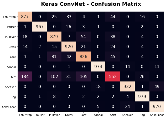
The ConvNet also struggled with “shirt” and did worse than LightGBM. It, however, did slightly better across the other categories. With comparable performance but significantly better fitting time, ConvNet is argumentively the better model.
ROC
fpr = dict()
tpr = dict()
roc_auc = dict()

for i, label in enumerate(label_index):
    fpr[i], tpr[i], _ = roc_curve(y_test_binarize[:, i], y_prob_keras[:, i])
    roc_auc[i] = auc(fpr[i], tpr[i])

fpr["micro"], tpr["micro"], _ = roc_curve(y_test_binarize.ravel(), y_prob_keras.ravel())
roc_auc["micro"] = auc(fpr["micro"], tpr["micro"])

all_fpr = np.unique(np.concatenate([fpr[i] for i in range(10)]))
mean_tpr = np.zeros_like(all_fpr)

for i in range(10):
    mean_tpr += np.interp(all_fpr, fpr[i], tpr[i])

mean_tpr /= 10

fpr["macro"] = all_fpr
tpr["macro"] = mean_tpr
roc_auc["macro"] = auc(fpr["macro"], tpr["macro"])

# Plot all ROC curves
plt.figure(figsize=(8,8))
plt.plot(fpr["micro"], tpr["micro"],
         label='micro-average ROC curve (area = {0:0.2f})'
               ''.format(roc_auc["micro"]),
         color='deeppink', linestyle=':', linewidth=4)

plt.plot(fpr["macro"], tpr["macro"],
         label='macro-average ROC curve (area = {0:0.2f})'
               ''.format(roc_auc["macro"]),
         color='navy', linestyle=':', linewidth=4)

for i, label in enumerate(label_index):
    plt.plot(fpr[i], tpr[i], lw=2,
             label=f'{label} (area = {round(roc_auc[i],2)})')

plt.plot([0, 1], [0, 1], 'k--', lw=2)
plt.xlim([0.0, 1.0])
plt.ylim([0.0, 1.05])
plt.xlabel('False Positive Rate')
plt.ylabel('True Positive Rate')
plt.title('Keras ConvNet - ROC curves of individual classes in Fashion MNIST')
plt.legend(loc="lower right")
plt.show()
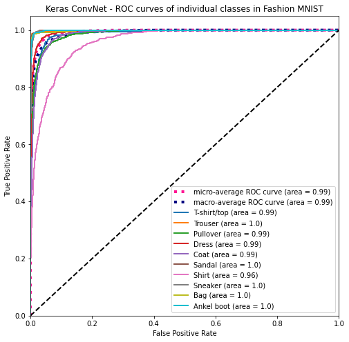
The ROC curve is also strikingly similar to the LightGBM’s model. With a 0.96 AUC, shirt is also the worse of the ten categories for ConvNet.
Conclusion
Both LightGBM and Keras’ ConvNet were able to achieve close to 90% accuracy with very basic techniques. Hyperparameter tuning would most certainly improve their accuracy.
tSNE is a very useful visualization tool for high dimensional dataset. It illustrated how it would be difficult to differentiate shirt from the other categories.