Forecasting Home Value with AutoARIMA
Follow along on Google Colab.
Introduction
“Of all the ways the ultra-rich made their fortunes, real estate outpaced every other method 3 to 1”, wrote Liz Brumer-Smith of Millionarces. Like any other investments, market knowledge is important for investing in real estates. Fortunately, with how widely available data is in today’s society, there are plenty of data that can be used to help make real estate investment decisions. In this exercise, future pricing of single family homes were prediced using data from Zillow.
This exercise was originally done as part of a course assignment for Big Data Analytics (IST 718) at Syracuse University.
Set Up
This notebook uses geopandas and pmdarima. It’s designed to run on Google Colab.
This notebook also uses two custom helpers; one to handle the data pull, and one to handle the times series.
Both of these custom helpers use multiprocessing to accelerate computation.
Install Libraries to Google Colab
geopandas is a geographical DataFrame manipulator and analytical library. contextily allows basemaps to be added to geospatial visuals. pmdarima is a time series analysis library.
The Runtime may have to be restarted after installing these libraries.
%pip install --upgrade geopandas
%pip install --upgrade pyshp
%pip install --upgrade shapely
%pip install --upgrade rtree
%pip install --upgrade matplotlib
%pip install --upgrade contextily
%pip install --upgrade pmdarima
%pip install --upgrade numpy
Cloning from Github
This clones the help functions from Github. This also clone the data needed to expedite the script.
!git clone https://github.com/lokdoesdata/zillow-forecast.git
import sys
sys.path.append(r'/content/zillow-forecast')
Import Libraries
%matplotlib inline
from helper import geom_data
from helper.time_series import TimeSeries
import pandas as pd
import geopandas as gpd
import matplotlib.pyplot as plt
import contextily as ctx
Data
The main dataset used in this exercise is from Zillow’s Housing Price Index by ZIP Code. This data set contains monthly housing price by ZIP Code. At the time of the analysis, there are data from January 1996 to March 2020.
An initial data inspection does not shows that the Zillow data set has a lot of incorrect state assigned to the ZIP codes. For example, ZIP code 00601 is assigned to Mississippi when it belongs to Puerto Rico. This mainly affect ZIP codes outside of the 50 states. However, external dataset can be used to correct them.
Two geodatabases from Esri were used:
- USA ZIP Code Areas which contains ZIP Code boundaries from TomTom (December 2019) and 2018 total population estimates from Esri demographics team.
- USA ZIP Code Points which contains ZIP Code points from TomTom December 2019 and 2018 total population estimates from Esri demographics team. This file is used for single site ZIP Codes.
One shapefile from the United States’ Census:
- Metropolitan and Micropolitan Statistical Area (MSA) from the 2010 Census (latest version at the time of analysis).
Zillow Data
The Zillow dataset was downloaded directly from Zillow.
df_zillow = pd.read_csv(r'https://files.zillowstatic.com/research/public/Zip/Zip_Zhvi_SingleFamilyResidence.csv')

df_zillow.drop([
    'RegionID',
    'SizeRank',
    'RegionType',
    'StateName',
    'State',
    'City',
    'Metro',
    'CountyName'
], axis=1, inplace=True)

df_zillow.rename({'RegionName': 'ZIP Code'}, axis=1, inplace=True)

df_zillow['ZIP Code'] = [str(z).zfill(5) for z in df_zillow['ZIP Code']]
Geographical Data
The geographical information for each ZIP code is processed using a helper module.
This could take a while due to the volume of data. This is also quite computational heavy.
gdf_zip_code = geom_data.get_zip_code_gdf()

gdf_zip_code.rename({
    'ZIP_CODE': 'ZIP Code',
    'PO_NAME': 'PO Name',
    'STATE': 'State',
    'POPULATION': 'Pop',
    'SQMI': 'Sq Mi',
    'NAME': 'MSA'
}, axis=1, inplace=True)

gdf_zip_code = gdf_zip_code[['ZIP Code', 'PO Name', 'State', 'Pop', 'Sq Mi', 'MSA', 'x', 'y', 'geometry']]

gdf_zip_code = gdf_zip_code.merge(df_zillow, on='ZIP Code')

del df_zillow
Converting the coordinate reference system to web mercator projection
gdf_zip_code = gdf_zip_code.to_crs(epsg=3857)
Exploratory Analysis
Choropleth map of home values by ZIP code
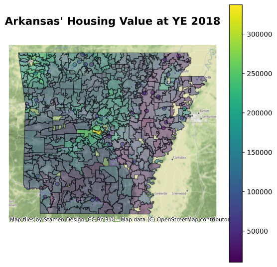
Arkansas was used as an illustration of a choropleth map of home values by ZIP code. The bright yellow spot in the center of Arkansas is ZIP code 72223. It has the highest median home value in Arkansas as of the end of 2018. This is a ZIP code in Little Rock, AR.
ax = gdf_zip_code[gdf_zip_code['State']=='AR'].plot(column='2018-12-31', figsize=(7, 7), legend=True, edgecolor='k', alpha=0.5)
ax.axis('off')
ax.text(x=0.5, y=1.1, s="Arkansas' Housing Value at YE 2018", fontsize=16, weight='bold', ha='center', va='bottom', transform=ax.transAxes)
ctx.add_basemap(ax)
Average home value by MSA
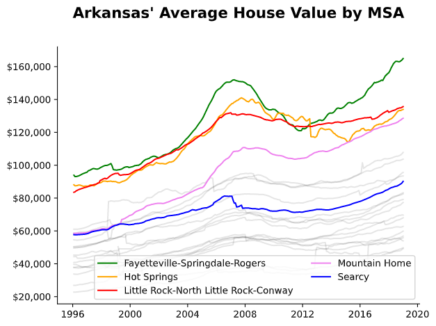
The average home value over time for Arkansas’ metropolitan and micropolitan areas with Fayetteville-Springdale-Rogers, Hot Springs, Little Rock, Mountain Home, and Searcy are highlighted. The non-highlighted lines are the average home values by MSA for the rest of Arkansas. The housing prices in Fayetteville-Springdale-Rogers, Hot Springs, Little Rock, and Mountain Home are a step above the rest of the state of Arkansas.
df_AR_MSA = gdf_zip_code[(gdf_zip_code['State']=='AR') & (gdf_zip_code['MSA']!='N/A')][['MSA'] + pd.date_range(start='1/1/1996', end='12/31/2018', freq='M').astype(str).tolist()].groupby('MSA').mean().T
df_AR_MSA.index = pd.to_datetime(df_AR_MSA.index)

color_dict = {
    'Little Rock-North Little Rock-Conway': 'red',
    'Hot Springs': 'orange',
    'Fayetteville-Springdale-Rogers': 'green',
    'Searcy': 'blue',
    'Mountain Home': 'violet'
}

f2, ax2 = plt.subplots(figsize=(7, 5))

for col in df_AR_MSA:
    ax2.plot(
        df_AR_MSA.index,
        df_AR_MSA[col],
        color=color_dict.get(col, 'k'),
        alpha=1 if col in color_dict.keys() else 0.1,
        label=col if col in color_dict.keys() else ''
    )

ax2.spines.right.set_visible(False)
ax2.spines.top.set_visible(False)
ax2.yaxis.set_major_formatter('${x:,.0f}')
ax2.yaxis.set_tick_params(which='major')
ax2.legend(loc='lower right', ncol=2)

ax2.text(x=0.5, y=1.1, s="Arkansas' Average House Value by MSA", fontsize=16, weight='bold', ha='center', va='bottom', transform=ax2.transAxes)
Time Series Forecasting
Model
The pmdarima package, and its stepwise approach, was used to train a SARIMA time series model for each ZIP Code. The general steps used to train each model is highlighted below:
- Determine the order of differencing (d) using a KPSS test.
- Determine the optimal auto regression (p) and moving average (d) with a maximum of five periods.
- With seasonal period (m) sets at 12 for monthly, determine the order of seasonal differencing (D) using a Canova-Hansen test.
- Determine the optimal seasonal auto regression (P) and seasonal moving average (Q) with a maximum of two periods.
- Select the optimal model based on Akaike information criterion (AIC), while ensuring that the model is numerically stable.
This was done with a train/test split with 2016 to 2018 data as training data and 2019 data as testing data. As such, only ZIP code with data between that time period were used in the analysis.
ts = TimeSeries(gdf_zip_code, '1/31/2019')
df_forecast = ts.forecast_all_states()
Results
The top 10 optimal seasonal ARIMA model is shown below:
df_forecast.model_order.value_counts().head(10)
| ARIMA Order | Number of ZIP Codes |
|---|---|
| ARIMA(0,1,0)(0,0,0)[12] intercept | 12,185 |
| ARIMA(0,2,0)(0,0,0)[12] | 2,087 |
| ARIMA(1,1,1)(0,0,0)[12] intercept | 1,282 |
| ARIMA(1,1,0)(0,0,0)[12] intercept | 1,029 |
| ARIMA(0,1,0)(0,0,1)[12] intercept | 932 |
| ARIMA(0,1,1)(0,0,0)[12] intercept | 652 |
| ARIMA(0,1,0)(1,0,0)[12] intercept | 644 |
| ARIMA(0,1,0)(0,0,0)[12] | 619 |
| ARIMA(0,1,0)(2,0,0)[12] intercept | 529 |
| ARIMA(2,1,2)(1,0,1)[12] intercept | 523 |
In summary, majority of the models are non-stationary, requiring differencing transformation. About half of the ZIP codes’ housing price is affected by seasonality.
ARIMA Example
Using ZIP Code 19124 as an example. The ACF plot shows a slow and steady decay, which suggests that the time series is non-stationary. A KPSSS test was also conducted and confirmed that two order of differencing is appropriate for this time series.
AutoARIMA determined that SARIMA(0,2,0)(0,0,0[12]) was the best model for this ZIP Code based on AIC. Please note that AIC cannot be compared directly for models with different orders.
Result
The profit and the ROI were calculated based on December 2018 actual housing value and December 2019 forecasted housing value.
df_investment = gdf_zip_code[['ZIP Code', 'x', 'y', 'PO Name', 'State', 'Pop', '2018-12-31']].merge(
    df_forecast[['zip_code', 'test_lci_2019-12-31', 'test_pred_2019-12-31', 'test_uci_2019-12-31']].rename({'zip_code':'ZIP Code'}, axis=1),
    on='ZIP Code'
)

df_investment.rename(
    {
        'Pop': 'Population',
        '2018-12-31': 'Before',
        'test_pred_2019-12-31': 'After',
        'test_lci_2019-12-31': 'After (Lower Bound)',
        'test_uci_2019-12-31': 'After (Upper Bound)',
    }, axis=1, inplace=True
)

df_investment['Profit'] = df_investment['After'] - df_investment['Before']
df_investment['ROI'] = df_investment['Profit']/df_investment['Before']
df_investment['Population'].fillna(0, inplace=True)
df_investment['Population'] = df_investment['Population'].astype(int)
df_investment['Name'] = [f'{p}, {s} {z}' for (p, s, z) in zip(df_investment['PO Name'], df_investment['State'], df_investment['ZIP Code'])]

df_investment = df_investment[['Name', 'x', 'y', 'Population', 'Profit', 'ROI', 'Before', 'After', 'After (Lower Bound)', 'After (Upper Bound)']]
Investment Opportunity
ZIP Code that provides the best real estate investment opportunity can be a challenging question. There are different ways to evaluate this and they come with different considerations.
Simple Helper Function
A simple helper functionw as created to help visualize the investment opportunity
# Simple helper function for plotting

def investment_plot(df, title):
    import seaborn as sns
    import matplotlib.pyplot as plt
    from matplotlib.lines import Line2D

    df = df.copy()
    df.reset_index(inplace=True, drop=True)

    f, ax = plt.subplots(figsize=(7, 7))
    ax.axis('off')

    with sns.axes_style('whitegrid'):
        sns.despine(left=True, bottom=True)
        for idx, row in df.iterrows():
            idx = idx*2
            ax.text(s='${:,.0f}k'.format(round(row['Before']/1000,1)), x=row['Before'], y=(-idx-0.1), horizontalalignment='right', verticalalignment='top')
            ax.text(s='${:,.0f}k'.format(round(row['After']/1000,1)), x=row['After'], y=(-idx-0.1), horizontalalignment='left', verticalalignment='top')
            ax.text(s='{} ({}% ROI)'.format(row['Name'], round(row['ROI']*100,1)), x=(row['Before']+row['After'])/2, y=-idx+0.15, horizontalalignment='center', verticalalignment='bottom')

            sns.scatterplot(x = [row['Before']], y = [-idx], color='red', ax=ax)
            sns.scatterplot(x = [row['After']], y = [-idx], color='green', ax=ax)
            sns.lineplot(x = [row['Before'], row['After']], y = [-idx, -idx], ax=ax, lw=2, color='black')

            ax.set_title(title, fontdict=dict(fontsize=16))

        legend_elements = [
            Line2D([0], [0], marker='o', color='w', label='Before', markerfacecolor='red'),
            Line2D([0], [0], marker='o', color='w', label='After', markerfacecolor='green'),
        ]
        ax.legend(handles=legend_elements, loc='lower right')


    return(df)
Return on Investment (ROI)
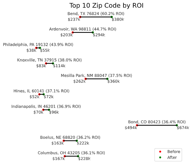
Based on return on investment, the three zip codes that provided the best real estate investment opportunity are:
- Bend, TX 76824
- Ardenvoir, WA 98811
- Philadelphia, PA 19132
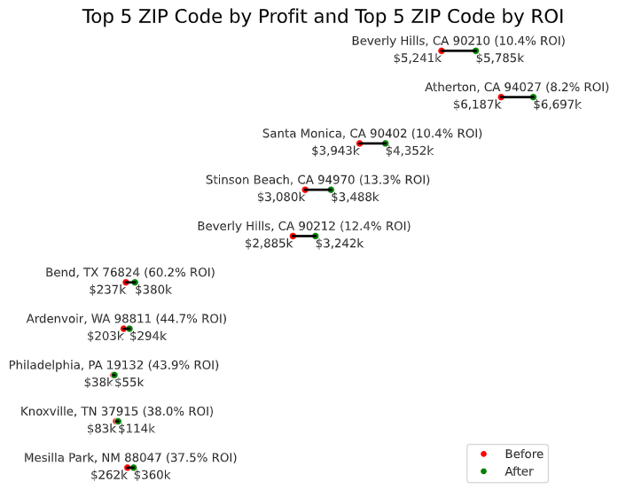
All three ZIP codes ziped over 40% ROI. However, looking at the population of Bend, and Ardenvoir with unrecorded population, suggested that there are not enough people in those ZIP codes for them to be worthwhile investment. Philadelphia, while having significant population, have limited profitability with only $16k per house.
investment_plot(df_investment.sort_values('ROI', ascending=False).head(10), 'Top 10 Zip Code by ROI')
| Name | x | y | Population | Profit | ROI | Before | After | After (Lower Bound) | After (Upper Bound) |
|---|---|---|---|---|---|---|---|---|---|
| Bend, TX 76824 | -98.523425 | 31.108534 | 0 | 142,730.32 | 0.602316 | 236,969.00 | 379699.32 | 366,535.97 | 392,862.68 |
| Ardenvoir, WA 98811 | -120.358272 | 47.731422 | 0 | 90,864.00 | 0.447093 | 203,233.00 | 294097.00 | 231,446.67 | 356,747.33 |
| Philadelphia, PA 19132 | -75.167859 | 39.996737 | 37,140 | 16,768.11 | 0.438577 | 38,233.00 | 55001.11 | 42,324.08 | 67,678.13 |
| Knoxville, TN 37915 | -83.901482 | 35.971976 | 6,421 | 31,392.00 | 0.380246 | 82,557.00 | 113949.00 | 87,467.16 | 140,430.84 |
| Mesilla Park, NM 88047 | -106.726674 | 32.223562 | 2,211 | 98,176.63 | 0.374985 | 261,815.00 | 359991.63 | 314,907.79 | 405,075.47 |
| Hines, IL 60141 | -87.839290 | 41.862194 | 278 | 19,378.00 | 0.370686 | 52,276.00 | 71654.00 | 57,427.14 | 85,880.87 |
| Indianapolis, IN 46201 | -86.106321 | 39.772938 | 31,897 | 25,879.17 | 0.369407 | 70,056.00 | 95935.17 | 82,527.93 | 109,342.40 |
| Bond, CO 80423 | -106.694352 | 39.905940 | 179 | 179,999.12 | 0.364169 | 494,273.00 | 674272.12 | 646,032.16 | 702,512.07 |
| Boelus, NE 68820 | -98.710625 | 41.102433 | 450 | 58,812.00 | 0.361608 | 162,640.00 | 221452.00 | 165,519.05 | 277,384.95 |
| Columbus, OH 43205 | -82.968058 | 39.957867 | 12,999 | 60,365.22 | 0.360963 | 167,234.00 | 227599.22 | 210,427.75 | 244,770.69 |
Profit
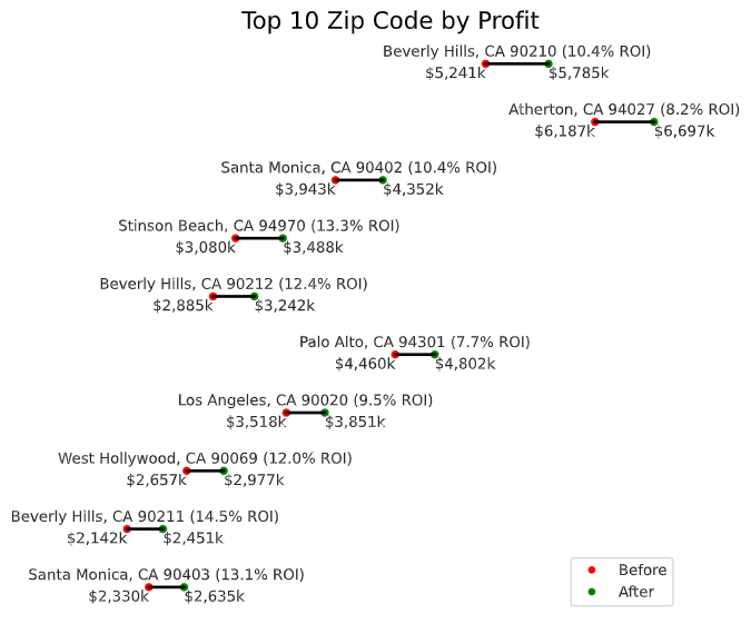
From a purely profit standpoint, the three most profitable ZIP Codes are:
- Beverly Hills, CA 90210
- Atherton, CA 94027
- Santa Monica, CA 90402
About half a million of profit is made per house in those three ZIP Code. However, those houses required signficiant upfront captial to purchase with close to $4M per house for the cheapest of the three ZIP Codes. This could be proven to be a real challenge for some investers without the necessary captials.
One additional note is that California made up of all the top 10 ZIP Codes in terms of profit.
investment_plot(df_investment.sort_values('Profit', ascending=False).head(10), 'Top 10 Zip Code by Profit')
| Name | x | y | Population | Profit | ROI | Before | After | After (Lower Bound) | After (Upper Bound) |
|---|---|---|---|---|---|---|---|---|---|
| Beverly Hills, CA 90210 | -118.399289 | 34.081401 | 24,230 | 543,504 | 0.103698 | 5,241,242 | 5,784,746 | 5,685,539 | 5,883,954 |
| Atherton, CA 94027 | -122.192663 | 37.458278 | 7,027 | 509,630 | 0.082372 | 6,186,961 | 6,696,591 | 6,481,279 | 6,911,902 |
| Santa Monica, CA 90402 | -118.507079 | 34.031337 | 12,447 | 409,184 | 0.103770 | 3,943,195 | 4,352,379 | 4,261,438 | 4,443,320 |
| Stinson Beach, CA 94970 | -122.649718 | 37.902736 | 721 | 408,392 | 0.132606 | 3,079,741 | 3,488,133 | 3,384,142 | 3,592,124 |
| Beverly Hills, CA 90212 | -118.399073 | 34.063506 | 12,610 | 356,692 | 0.123623 | 2,885,330 | 3,242,022 | 3,177,961 | 3,306,082 |
| Palo Alto, CA 94301 | -122.153657 | 37.443679 | 18,461 | 342,138 | 0.076721 | 4,459,512 | 4,801,650 | 4,512,463 | 5,090,837 |
| Los Angeles, CA 90020 | -118.301614 | 34.066172 | 40,967 | 332,700 | 0.094559 | 3,518,436 | 3,851,136 | 3,251,457 | 4,450,815 |
| West Hollywood, CA 90069 | -118.382874 | 34.089240 | 21,120 | 319,686 | 0.120307 | 2,657,244 | 2,976,930 | 2,918,801 | 3,035,058 |
| Beverly Hills, CA 90211 | -118.382430 | 34.066743 | 9,219 | 309,528 | 0.144513 | 2,141,866 | 2,451,394 | 2,159,287 | 2,743,501 |
| Santa Monica, CA 90403 | -118.492328 | 34.028155 | 25,766 | 304,666 | 0.130743 | 2,330,269 | 2,634,935 | 2,592,932 | 2,676,939 |

When the ZIP codes with most raw profit are ZIP Codes with the most ROI are stacked on top of one another, it clearly shows that getting lesser ROI in a more expensive area is a better investment than higher ROI in a less expensive area.
| Name | x | y | Population | Profit | ROI | Before | After | After (Lower Bound) | After (Upper Bound) |
|---|---|---|---|---|---|---|---|---|---|
| Beverly Hills, CA 90210 | -118.399289 | 34.081401 | 24,230 | 543,504 | 0.103698 | 5,241,242 | 5,784,746 | 5,685,539 | 5,883,954 |
| Atherton, CA 94027 | -122.192663 | 37.458278 | 7,027 | 509,630 | 0.082372 | 6,186,961 | 6,696,591 | 6,481,279 | 6,911,902 |
| Santa Monica, CA 90402 | -118.507079 | 34.031337 | 12,447 | 409,184 | 0.103770 | 3,943,195 | 4,352,379 | 4,261,438 | 4,443,320 |
| Stinson Beach, CA 94970 | -122.649718 | 37.902736 | 721 | 408,392 | 0.132606 | 3,079,741 | 3,488,133 | 3,384,142 | 3,592,124 |
| Beverly Hills, CA 90212 | -118.399073 | 34.063506 | 12,610 | 356,692 | 0.123623 | 2,885,330 | 3,242,022 | 3,177,961 | 3,306,082 |
| Bend, TX 76824 | -98.523425 | 31.108534 | 0 | 142,730.32 | 0.602316 | 236,969.00 | 379699.32 | 366,535.97 | 392,862.68 |
| Ardenvoir, WA 98811 | -120.358272 | 47.731422 | 0 | 90,864.00 | 0.447093 | 203,233.00 | 294097.00 | 231,446.67 | 356,747.33 |
| Philadelphia, PA 19132 | -75.167859 | 39.996737 | 37,140 | 16,768.11 | 0.438577 | 38,233.00 | 55001.11 | 42,324.08 | 67,678.13 |
| Knoxville, TN 37915 | -83.901482 | 35.971976 | 6,421 | 31,392.00 | 0.380246 | 82,557.00 | 113949.00 | 87,467.16 | 140,430.84 |
| Mesilla Park, NM 88047 | -106.726674 | 32.223562 | 2,211 | 98,176.63 | 0.374985 | 261,815.00 | 359991.63 | 314,907.79 | 405,075.47 |
Population as a factor
Population can be a sign of potential home buyers in a ZIP code. While profitability is important, they need to be in area with potential home buyers.
gdf_investment_top1k = df_investment.sort_values('Profit', ascending=False).head(1000)
gdf_investment_top1k = gpd.GeoDataFrame(
    gdf_investment_top1k,
    geometry=gpd.points_from_xy(gdf_investment_top1k.x, gdf_investment_top1k.y)
)
gdf_investment_top1k = gdf_investment_top1k.set_crs(4326).to_crs(3857)
Most profitable ZIP codes
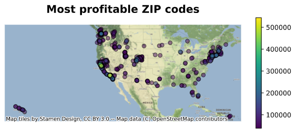
The most profitable ZIP codes are shown in the figure below. California looks to be filled with profitable ZIP codes, followed by New York and its surrounding areas.
ax3 = gdf_investment_top1k.sort_values('Profit').plot(
    column='Profit', figsize=(8, 3), legend=True, edgecolor='k', alpha=0.5)

ax3.axis('off')
ax3.text(x=0.5, y=1.1, s='Most profitable ZIP codes', fontsize=16, weight='bold', ha='center', va='bottom', transform=ax3.transAxes)
ctx.add_basemap(ax3)
Population of the most profitable ZIP codes
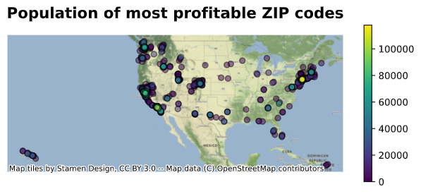
The population of the most profitable ZIP codes in the above figure is shown below. Both California and New York have sizeable population.
ax4 = gdf_investment_top1k.sort_values('Population').plot(
    column='Population', figsize=(8, 3), legend=True, edgecolor='k', alpha=0.5)

ax4.axis('off')
ax4.text(x=0.5, y=1.1, s='Population of most profitable ZIP codes', fontsize=16, weight='bold', ha='center', va='bottom', transform=ax4.transAxes)
ctx.add_basemap(ax4)
Conclusion
While return on investment is an important metric for any type of investment, it is important to not overlook at the potential profit that can be made in a market. In a simplified way, there are two main factors to determine the size of the market; how much does a home cost, and how many homes can be sold? Using the median housing price and the population data, it was determined that if there is enough initial capital, California is the best place to invest for real estates.